Raphaël Kanapitsas

The Wave Equation

Still in the process of being written.

Disclaimer: math-heavy article, on a topic I learnt about by writing: it might contain errors. Please comment if you see anything not making sense!

The other day, I looked at my guitar, and realized that I didn't known how waves behave on a string, mathematically speaking. How do they propagate? The string is fixed between two points. You pluck the string, by displacing it at a certain point, and letting go. What happens then?

Derivation

Imagine a string with tension $T$, linear mass density $\mu$. We consider only the vertical displacements of the string, which should stay small (like on a string instrument). We will model our string as a function $y$, that gives the vertical displacement given coordinate $x$ and time $t$.

$$\begin{align} y: [0,L] \times \mathbb R^+ &\longrightarrow [-y_\text{max}, y_\text{max}] \\ (x, t) &\longmapsto y(x,t) \end{align}$$

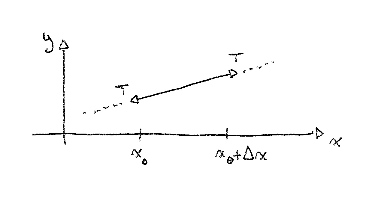
Let's forget time for now, and look at static situations. Here's a piece of string with tension acting on it on both ends.

Not much is happening here: the string is straight, the forces acting on it even out, everything stays in place. But let's look at what happens when there's some curvature.

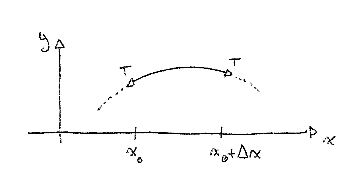Here, we imagine the net force would make the piece of string go downwards. We can find the mass of the piece easily: $m_{\Delta x} = \mu \Delta x$. If we can find the net force acting on it, we'll be able to apply Newton's second law.

We've made the assumption that the movement of the string is only in the $y$ direction. This means we can consider only the vertical forces acting on the piece, at $x_0$ and $x_0 + \Delta x$.

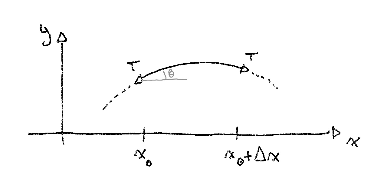
From this picture, we can see that the vertical fore acting at $x_0$ is $F_{x_0} = -T \sin(\theta)$. Knowing that the $y$ displacements are small, we can make the small angle approximation physicists love, and use the slope instead of $\sin$ ¹, and get:

$$F_{x_0}=-T \frac{d}{dx}y(x_0)$$ We can find the force from the other end the same way²: $$F_{x_0+\Delta x}=T \frac{d}{dx}y(x_0+\Delta x)$$

We can sum them and get the net force acting on this small piece of string. $$F_\text{net} = T\left( \frac{d}{dx}y(x_0+\Delta x) - \frac{d}{dx}y(x_0) \right)$$ Great! We have everything we need to apply Newton's second law. Let's also put back time into the equation. $$T\left( \frac{\partial}{\partial x}y(x_0+\Delta x, t) - \frac{\partial}{\partial x}y(x_0, t) \right) = F_{x_0,t} = m_{\Delta x} a_{x_0,t} = \mu \Delta x \frac{\partial^2}{\partial t^2}y(x_0,t)$$ Reorganizing a bit: $$T\frac{ \frac{\partial}{\partial x}y(x_0+\Delta x, t) - \frac{\partial}{\partial x}y(x_0, t)} {\Delta x} = \mu \frac{\partial^2}{\partial t^2}y(x_0,t)$$ Supposing our function $y$ is well-behaved, we have: $$\frac{ \frac{\partial}{\partial x}y(x_0+\Delta x, t) - \frac{\partial}{\partial x}y(x_0, t)} {\Delta x} \xrightarrow[\Delta x \to 0]{} \frac{\partial^2}{\partial x^2}y(x_0, t)$$ In the end, taking a general $x$ instead of $x_0$, our equation becomes:

$$T \frac{\partial^2}{\partial x^2}y(x, t) = \mu \frac{\partial^2}{\partial t^2}y(x, t)$$ Or, as it is more often presented: $$\frac{\partial^2}{\partial t^2}y(x, t) = \frac T \mu \frac{\partial^2}{\partial x^2}y(x, t)$$ This reflects well our early intuition that the more curved the string is at some point, the faster it would move. The higher the tension, the faster, the higher the mass density, the slower. Sanity check: pass.

We can do two things from here, now that we have this partial differential equation: we can stop here, and go simulate it on a computer, or we can try to find explicit solutions.

Solutions

Of course, this equation is ideal, in that it doesn't reflect all of reality. For example, there's no damping, and a movement will continue forever. But it's still useful to understand how waves propagate in this environment, especially if we can find the general form of the solutions.

Separation of variables

Let's try to simplify the problem by "trying out" the assumption that $y$ can be written as the product of two simpler functions, each depending on only one parameter:

$$y(x,t) = X(x) T(t)$$

This severely simplifies the problem and limits the number of forms that $y$ can take. Let's substitute $y$ for this product in the wave equation:

$$\begin{align} \frac{\partial^2}{\partial t^2}y(x, t) &= \frac T \mu \frac{\partial^2}{\partial x^2}y(x, t) \\ \frac{\partial^2}{\partial t^2}[X(x)T(t)] &= \frac T \mu \frac{\partial^2}{\partial x^2}[X(x)T(t)] \\ X(x)T''(t) &= \frac T \mu X''(x)T(t) \end{align}$$ When $X(x) \neq 0$ and $T(t) \neq 0$, we can rearrange a bit³ $$\frac{T''(t)}{T(t)} =\frac T \mu \frac {X''(x)}{X(x)}$$ Each side depends only on one variable, which means they are both equal to the same constant!

Solving each side

Let's take the left-hand side first

$$\begin{align} \frac{T''(t)}{T(t)} &= \alpha\ \in \mathbb R \\ T''(t) &= \alpha T(t) \end{align}$$ If we're looking for a function whose derivative is almost the same, we're looking at the exponential. Let's set $T(t) = e^{at}$. We get that: $$a^2 e^{at} = \alpha e^{at} \iff a^2 = \alpha$$ If $\alpha > 0$, we have $T(t) = e^{\sqrt{\alpha} t}$, but we're probably not looking for an exponential function, as it won't satisfy our boundary conditions. On the other hand, if $\alpha < 0$, we have $T(t) = e^{\pm it\sqrt{-\alpha}}$, which looks a lot more like the waves we've been talking about.

It makes sens intuitively: if $T''(t)/T(t) > 0$, the function has a positive curvature when it's already positive, making it grow even more. In the other case, it has a negative curvature, which is more reminiscent of the restoring force we found in the first part.

For simplicity, let's set $\alpha = -k^2$, so that we have: $$T(t) = e^{\pm ikt}$$ We can follow the exact same procedure for $X$, which is the same equation with a additional multiplicative constant. $$X''(x) = -k^2 \frac \mu T X(x)$$ and try $X(x) = e^{b x}$ $$b^2 e^{b x} = -k^2 \frac \mu T e^{b x} \iff b^2 = -k^2 \frac \mu T$$ So that $b = \pm ik \sqrt{\frac \mu T}$ . Let's define $\lambda = k \sqrt \frac \mu T$ for simplicity.

Our two resulting "elemental" solutions (actually four, counting the signs) are: $$\begin{align} T(t) &= e^{\pm ikt} \\ X(x) &= e^{\pm i \lambda x} \end{align}$$ But the equation is linear, meaning that any linear composition of these is still a solution. That means our general form is:

$$y(x,t) = X(x)T(t) = (A_1 e^{i \lambda x} + B_1e^{-i \lambda x}) (A_2 e^{ikt} + B_2e^{-ikt})$$ Where $A_1, A_2, B_1, B_2 \in \mathbb C$

Applying the boundary conditions

Spatial

We are ready to apply some boundary conditions. First, the string is fixed in place at $x=0$ and $x=L$, which means that $\forall t$ we have $y(0,t) = y(L,t) = 0$. The first one translates to: $$y(0,t) = X(0)T(t) = (A_1+B_1)(A_2 e^{ikt} + B_2 e^{-ikt}) = 0$$ So at least one of the member is null. For the right side to be null would mean that $A_2 = B_2 = 0$ which leads to a non-moving string. Other wise, we have $B_1 = -A_1$, and $$\begin{align} X(x) &= A_1 (e^{i \lambda x} -e^{-i\lambda x}) = 2i A_1 \sin(\lambda x) \\ &= C \sin(\lambda x) \end{align}$$ Applying the condition from the other end of the string, we get: $$X(L) = C \sin(\lambda L) = 0 \iff \lambda L=n\pi \iff \lambda=\frac{n\pi}{L}$$ Which is valid for any $n \in \mathbb N^*$, meaning $X$ can be a superposition of those: $$X(x) = \sum_{n\in\mathbb N^*} C_n \sin\frac{n\pi}{L} x$$

Temporal

If we consider the movement of a guitar string, at the initial pluck, the velocity of the string is $0$ everywhere (before the player lets the string go). Which means that $T'(0) = 0$: $$\begin{align} T'(t) &= ikA_2 e^{ikt} - ikB_2 e^{-ikt} \\ T'(0) &= ikA_2 - ikB_2 = 0 \iff A_2 =B_2 \end{align}$$ We can now simplify the writing of $T$: $$\begin{align} T(t) &= A_2(e^{ikt}-e^{-ikt}) = 2A_2 \cos(kt) \\ &=D \cos(kt) \end{align}$$ We also know that $k=\lambda \sqrt \frac T \mu = \frac{n\pi} L \sqrt \frac T \mu$, which means we also have a superposition here: $$T(t) = \sum_{n \in \mathbb N^*} D_n \cos\sqrt \frac T \mu \frac{n\pi} L t$$

Final solution

By combining these terms, with new $a_n=C_n+D_n$, we have⁴

$$y(x,t) = \sum_{n\in\mathbb N^*} a_n \sin \left( \frac{n\pi x} L \right) \cos \left( \sqrt \frac T \mu \frac{n\pi t} L\right)$$ And by applying $\sin(x)\cos(y) = \frac 1 2 (\sin(x+y) + \sin(x-y))$ we get $$y(x,t) = \frac 1 2 \sum_{n \in \mathbb N^*} a_n \left( \sin \frac{n\pi}{L}\left(x+ t\sqrt \frac T \mu \right) + \sin \frac{n\pi}{L}\left(x- t\sqrt \frac T \mu \right) \right)$$ Which is a more interpretable form of the solutions: for each frequency, there's a wave going to the right, and another going to the left. In this form, we can also see that $c = \sqrt \frac T \mu$ is the speed at which the wave propagates. Let's re-write it with that simplification in mind:

$$y(x,t) = \frac 1 2 \sum_{n \in \mathbb N^*} a_n \left( \sin \frac{n\pi}{L}\left(x+ ct \right) + \sin \frac{n\pi}{L}\left(x- ct \right) \right)$$ Actually, we still have an unknown, or rather an infinity of them, namely all the $a_n$s. But these can be determined with the initial state of the string $y(x, 0)$. If we plug that in, we obtain: $$y(x, 0) = \sum_{n\in\mathbb N^*} a_n \sin \left( \frac{n\pi x} L \right)$$ Which is just the Fourrier decomposition of the initial state.

(TODO add explanation about Fourrier series)

$$a_n = \frac 2 L \int_0^L y(x,0) \sin \frac {n\pi x} L dx$$ Read more here

Simulation

Now a bit of fun. By making the domain (both temporally and spatially) discrete, we can model the string at time $t$ by an array $\tilde{y}_t \in \mathbb R^n$, where $n = \frac L {\Delta x}$ and $\Delta x$ is the spatial definition. We can keep track of the vertical speed of the string at any point with another array $\tilde{v}_t \in \mathbb R^n$.

This way, we can keep track of the system at time $t$, and update it based on the previous equation. This is done using a finite-difference approximation of the second spatial derivative (which is just the approximation you get by considering the definition of a derivative)

$$\frac {\partial^2}{\partial x^2} y(x,t) \approx \frac {y(x-\Delta x, t) - 2y(x, t) + y(x+ \Delta x, t)} {\Delta x^2}$$ From this, using the wave equation, we get an approximation $\tilde{a}(x,t)$ of acceleration. Integrating once is easily approximated: $$\int_t^{t+\Delta t} \tilde{a}(x, t) dt \approx \tilde{a}(x, t) \Delta t =: \Delta \tilde{v}_t$$ This gives us the change of speed, with which we can update our $\tilde{v}_{t+\Delta t} \leftarrow \tilde{v}_t + \Delta \tilde{v}$ and by "integrating" again...

$$\int_t^{t+\Delta t} \tilde{v}(x, t) dt \approx \tilde{v}_t \Delta t =: \Delta \tilde{y}_t$$

...we get an update to our $y$ by doing $\tilde{y}_{t+1} \leftarrow \tilde{y}_t + \Delta \tilde{y}_t$ and the cycle starts again, approximating the new position and speed at each time step. Of course, all that is of no use if we don't get to see it in action!

Comparison with a real string